1. Introduction

    With rapid progress of the information age, information itself as well as physical objects has become a major part of economic value and current popularity of information technology (IT) intensifies the importance of information. For example, in the manufacturing industries, products are mostly represented in digital form at the design stage, and the digital information of the products becomes an essential element in fabrication.

    In the past, such 3-D model description had been presented with a fairly restrictive format such as 2-D drawings, i.e. blueprints. Today, these 3-D objects are typically described with computer-aided design (CAD) systems using digital data. Here, the richest shape variety can be described using free-form boundary surfaces that are typically defined by Non-Uniform Rational B-spline (NURBS) surface patches.

    Digital data models describing objects are often accessible to various parties. This occurs, for example, when the detailed design specifications are shown to prospective buyers of a physical copy of the object. Furthermore, the digital model data could be known to another party, e.g. a subcontractor or by industrial espionage, e.g., when data are communicated via the Internet. It is also possible that a party could approximate digital model data by reconstructing the geometric model by reverse engineering a single physical prototype. In other instances, there could be a need for several engineers working together to simultaneously access a design database and to make changes in the database that are instantly accessible by others on the team. At the same time, there is a need for conveying these data to designers at remote locations while providing a high level of security on proprietary designs. Especially, when proprietary digital content is exposed to the Internet, it can become an easy target for malicious parties who wish to reproduce unauthorized copies. For these reasons, protection of digital intellectual property has become an active research topic and many people have begun to research digital watermarking methods.

    Several methods have been reported on digital watermarking for 3-D polygonal models that are widely used for virtual reality and computer graphics. Most of the methods are designed for triangle meshes and embed watermark information by perturbing geometry or changing topological connectivity [13,21,1] or using the frequency domain of 3-D models for embedding watermarking information [6,17,22].

    Watermarking on Constructive Solid Geometry (CSG) models was developed by Fornaro and Sanna [4]. An extractable watermark is built using a hash function, and a public key algorithm is used for encryption and decryption of the watermark. Two places are considered for storing the watermark: solid and comment nodes. To store the watermark in the solid, a new watermark node is created and linked to the original CSG tree. In the comment nodes, the watermark information can be added without change of the model.

    Despite the popularity of NURBS curves and surfaces, watermarking for NURBS representations is relatively new to engineering CAD. Ohbuchi et al. [14] proposed a new data embedding algorithm for NURBS curves and surfaces, which are reparameterized using rational linear function whose coefficients are manipulated for encoding data. The exact geometric shape is preserved. The watermark information, however, can be easily destroyed by reparameterization or reapproximation of the surface.

    In this project, we developed efficient computational algorithms and criteria for comparing two objects represented in NURBS form or 3-D B-rep solids so that one can determine if one is a duplicate of the other. Surface intrinsic properties are used to make the algorithms independent of representation methods, scaling, rotation and transformation and use of generic umbilical points for comparison enhances robustness of the algorithms with respect to small perturbations.

    This paper is structured as follows. In section 2, algorithms are introduced with detailed explanation of computational methods. Section 3 demonstrates the algorithms with a few examples and Section 4 concludes the paper.

 

2. Overview of Shape Intrinsic Watermarking

Two 3-D objects are provided for comparison. One of them is an original model denoted as A and the other is a suspect denoted as B.

Assumptions

(1)     Representation form 

a.        A and B are solids 

                                                      i.      They are represented via a boundary representation (B-rep) scheme and the surfaces of the two B-rep models are homeomorphic (they have the same genus G or number of handles).

                                                     ii.      The surfaces which bound the solids are of NURBS form. 

b.       A and B are surfaces 

                                                      i.      They are represented in NURBS form.

(2)     After applying uniform scaling, rotation and translation to one object, the difference of the two objects as point sets is small.

(3)     All kinds of geometrical operations including translation, rotation, uniform scaling, perturbation of control points, reparameterization, etc. have been imposed on B. The operations such as shearing and non-uniform scaling, which degrade the appearance or functionality of the object, however, are not included. 

2.1. Preliminary Step

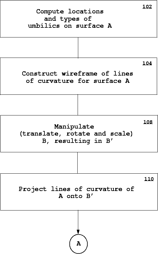
 Before checking the similarity of two objects, a sequence of operations needs to be performed. Four operations are proposed in Figure 1, and explained in subsequent sections of this paper.  After this step, the object A and localized (translated, rotated and scaled) solid B^’ are available for input to the comparison algorithms.

 

Figure 1: A Preliminary step (Clikc here for a larger image.)

2.1.1. Detection and Classification of Umbilics

An umbilical point is a point on a surface where all the normal curvatures are equal in all directions. All the points in planar and spherical surface regions are umbilics. There are two categories of isolated umbilics: one is generic and the other is non-generic. Generic umbilics are stable with respect to small perturbations of the function representing the surface, while non-generic umbilics are unstable [2,18,20,12,15].

    Generic umbilics have three different types called star, (le) monstar and lemon based on the pattern of the lines of curvature in the vicinity of the umbilics as shown in Figure 2. They are stable with respect to small perturbations of the surface. An input NURBS surface is decomposed into rational Bézier patches using the knot insertion technique and each rational Bézier patch is supplied to set up governing equations. The governing equations for locating umbilics consist of three polynomial equations with two unknowns when input surfaces are in integral/rational Bézier forms. The system of nonlinear polynomial equations can be solved robustly and accurately by the Interval Projected Polyhedron (IPP) algorithm [19,15]. One line of curvature passes for the lemon type umbilical point whereas three pass throught the umbilical point of monstar or star types. The criterion distinguishing between monstar and star types is that all three directions of lines of curvature through a monstar umbilic are contained in a right angle, whereas in the star type umbilical point case, they are not enclosed in a right angle [12]. Given two umbilical points of same type i.e. star type, then we can compute the distributions of the angles formed by two consecutive lines of curvature at the umbilical points. Using the distributions, two umbilical points of same type can be distinguished. For more details, see  [12,15].

 

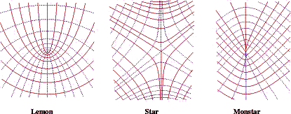
Figure 2: Three generic umbilics adopted from [15]

2.1.2. Shape Intrinsic Wireframing

Computation of Orthogonal Net of Lines of Curvature

A curve on a surface whose tangent at each point is in a principal curvature direction is called a line of curvature [12]. At each point there are two principal directions (maximum and minimum) that are orthogonal so that the corresponding lines of curvature form an orthogonal net of lines. Lines of curvature are intrinsic to the surface and do not depend on coordinate transformations and parameterization of the surface. The same orthogonal net of lines is always obtained as long as the surface shape remains unchanged.   

   Lines of curvature on a parametric surface can be computed from a set of differential equations with respect to the arc length. An integration method such as fourth order Runge-Kutta method or Adam’s method with variable step size may be used to find the solution [3,12].

Computation of Geodesic Curves

Some areas do not allow us to construct an orthogonal net of lines of curvature such as near boundary and umbilical points. In such areas, another surface intrinsic property, geodesic curves, may be employed for completion of the wireframe. A geodesic curve is defined as a curve whose geodesic curvature is zero. In general, it arises as the boundary value problem (BVP) so that when two points are provided, a geodesic curve is calculated which connects them. For a stable solution, the relaxation method is adopted for the computation of the geodesic curve. For details, see [15,10].

 

Algorithm

 

An algorithm for the construction of intrinsic wireframing is shown in Figure 3.

 

 

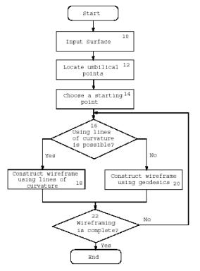
Figure 3: A diagram of the algorithm

 

Steps 10 and 12 : Input Surfaces and Umbilics

The algorithm needs to be provided with information on exact locations of umbilical points over an input surface to trace lines of curvature properly using the method in Step 18 since lines of curvature cannot be uniquely determined at umbilical points, which can be computed and classified by using the methods in Section 2.1.1.

 

 Step 14 : Starting Points

Either a star type umbilical point or a non-umbilical point can be chosen as a starting point for wireframing because the maximum and minimum lines of curvature radiate from the point in an alternating pattern so that a simple algorithm is sufficient and the resulting mesh is more well-proportioned. The other two types of umbilics, i.e. lemon and monstar, are not appropriate for this purpose. At a star type umbilical point, there are three lines of curvature each of which changes its attribute from the maximum to the minimum or vice versa. Therefore, six lines of curvature are considered to radiate from the umbilical point so that we can use up to six initial directions for tracing lines of curvature. When there is no umbilical point on the surface, a non-umbilical point is chosen as a starting point where four initial directions for tracing are obtained.

 

Step 18 : Wireframing with Lines of Curvature

Surface intrinsic wireframe representation is constructed with lines of curvature which are calculated by using any popular numerical methods such as the fourth order Runge-Kutta method from starting points determined in Step 14. In most cases, maximum and minimum lines of curvature form quadrilateral meshes. Therefore, the important step in creating a wireframe with lines of curvature is to locate intersection points between maximum and minimum lines of curvature.  These points can be accurately computed using Newton’s method.

 

Step 20 : Geodesic Wireframing

In a region where the algorithm using lines of curvature fails, i.e. in the neighborhood of an umbilical point (except the umbilical point used as a starting point) and near boundary or in an umbilical region, a geodesic curve can be used to complete wireframing. Two points are selected and a geodesic line is  calculated which connects them. As an initial approximation, a straight line connecting two boundary points is used, from which an accurate solution is obtained iteratively by using the relaxation method, see [10, 15].

 

In Figure 4, an example of shape intrinsic wireframing is presented. The construction of the wireframe starts from the star type umbilical point in the center using lines of curvature. Geodesic curves are used in the regions that the lines of curvature do not cover. Since it only depends on the shape of the input surface, the same wireframe can be obtained irrespective of representation.

 

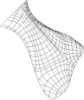
Figure 4: An example of shape intrinsic wireframing

 

2.1.3. Matching

Matching is a process determining a rigid body motion (translation and rotation) which makes two objects match as closely as possible. Three methods for matching are used: the moment method, the KH method and the umbilical point method. The moment method is a global method and used for solid matching. The other two approaches are to use intrinsic properties on the surface of objects. The KH method uses curvature information and the umbilical point method is based on generic umbilical points on the surface of objects. These two methods can be applied not only to global matching but also to partial matching.

Integral Property

Matching via integral properties is used for solids. The integral properties for solid A and B i.e. centroids (centers of volume) and moments of inertia, are calculated using Gauss’s theorem or the divergence theorem which reduces volume integrals to surface integrals. The inertia tensors of solid A and B are constructed. The inertia tensor consists of a 3x3 symmetric square matrix whose terms on the main diagonal I_xx, I_yy and I_zz are called the moments of inertia and the remaining terms (I_xy , I_yx , I_xz , I_zx , I_yz  and I_zy) are called the products of inertia. Because of symmetry, it is always true that I_xy = I_yx, I_xz = I_zx and I_yz = I_zy. Principal moments of inertia and their directions are obtained by solving an eigenvalue problem. Once the centroids and principal directions of both solids are calculated, solid A and B are translated and rotated so that their centroids and principal axes of inertia coincide. Solid B is uniformly scaled based on the volume ratio of the two solids.

KH Method

Two surface intrinsic properties, the Gaussian and mean curvatures, are used for localization purposes. Three points are selected on the surface of the object B and three pairs of the Gaussian and mean curvatures are calculated there. Then the corresponding points which have the same Gaussian and mean curvatures calculated on the object B are located by solving a system of equations formulated for the object A using the Interval Projected Polyhedron algorithm. After the correspondence has been established, a rigid body motion is calculated which aligns two objects as closely as possible. This method works well when no initial correspondence information is available and only partial surfaces are provided. For details, see Ko et al. [7].

Umbilical Point Method

This paper employed ensembles of isolated umbilical points that have stable patterns useful to recognize that a surface patch had been obtained by a small perturbation of another surface patch having an equivalent collection of finitely many (isolated) stable umbilical points. Our proposal involving use of the "pattern of stable umbilical points" in order to support the recognition of surface patches may raise some questions concerning its usefulness. The reason for those doubts is that if we consider surfaces that are infinitely often continuously differentiable then the structure of their respective sets of umbilical points may be quite complicated. Within the family of general infinitely often differentiable surfaces it is possible to construct very small perturbations that will change surfaces having only finitely many (stable) umbilics into new surfaces having infinitely many isolated stable umbilical points that may occur in quite complex geometric arrangements.  (Here a simple construction of surface with infinitely many isolated stable umbilics may e.g. be achieved by attaching a sequence of infinitely many very small shrinking bumps to a cylindrical surface patch.) The latter construction and complex arrangements of umbilical points are possible due to the fact that the differentiability class C^¥ still allows e.g. all kinds of infinitely many arbitrarily small local perhaps oscillatory surface deformations. However, if we restrict our attention to Bézier or B-spline surface patches of limited degree then the number of isolated umbilical points is limited as well.  Here the maximal number of isolated umbilical points existing on the Bézier surface patch can be estimated from above using the degree information of the Bézier surface patch or the information on the number of control points. A similar estimation is possible for B-spline surface patches as well. Hence working with Bézier surface patches yields a finiteness condition for the number of umbilics.  In case we perturb e.g. the Bézier surface patch within the family of Bézier surface patches of the same degree, then we shall obtain new patches with a finite maximal number of isolated umbilics as well. The latter maximal number has the same bound as the one being valid for the unperturbed Bézier surface patch. Such a surface perturbation can be realized by deforming the original surface patch via perturbing all control points of the original Bézier surface patch, see [12]. Such perturbations are very specialized and restrictive in comparison to the general case where we may consider general surfaces that have regular parametrizations being infinitely often differentiable. However, from a practical point of view the restriction to the family of Bézier surface patches even with degree restrictions is justified in an engineering context. Hence, here it is practically correct to consider only the restricted metamorphosis -possibilities- of an ensemble of finitely many stable umbilics located on the original Bézier surface patch. This definitely excludes inconvenient pathologies that would otherwise be possible. Moreover the preceding considerations should help to illuminate a posteriori why the diagnostic tool employing the pattern of (finitely many) isolated stable umbilics is relevant in supporting the diagnosis that a Bézier surface patch is obtained via a fairly small deformation (within the Bézier family) from the given original Bézier surface patch.

 

When isolated generic umbilical points exist on the surfaces of two objects, they can be used to establish correspondence between the objects. Conceptually, a matching algorithm using generic isolated umbilical points is straightforward. The basic idea is to find a pair of umbilical points which have the same type. Each type can be distinguished by the methods described in Section 2.1.1. If we have more than three matching pairs of umbilical points, then we can easily find a rigid body transformation in the least squares sense. When there are less than two pairs, we match the normal vectors and align the radiating patterns of lines of curvature at the corresponding umbilical points. In most cases, the number of generic isolated umbilical points is small. Therefore, a brute force search scheme to find matching pairs of umbilical points can be employed without loss of performance. See Ko et al. [8] for details.

Matching with Scaling Effects

Two methods are proposed to resolve uniform scaling in global and partial matching. One is based on the umbilical point method and the other is to formulate a matching problem as an optimization problem using the KH method. In case of global matching, a scaling value may be recovered by calculating the ratio of areas between two surfaces or volumes between two objects. However, for partial matching, comparison of any kinds of quantitative measures does not make sense. Only qualitative feature matching or searching a good match from a set of candidate solutions can be considered. See Ko et al. [8] for details.

 

Searching a pair of corresponding umbilical points can be performed irrespective of scaling effects since the qualitative aspects of umbilical points are used for finding corresponding umbilical points. Once a pair of the umbilical points are found, the normal curvature values at the umbilical points can be used to estimate a scaling factor.

 

Matching with scaling effects is formulated as an optimization problem. The KH method can be treated as an objective function of the scaling factor. Namely, under a certain scaling value, we can apply the KH method to the objects under consideration. Then the KH method computes a value which represents the sum of the Euclidean distances between two objects. This process manifests itself as an optimization problem and we can employ any optimization solution method to find a scaling factor as well as a rigid body transformation with which the KH method produces the minimum value.

2.2. Matching Conditions

Computational methods and criteria are proposed that allow us to check the similarity of two objects.  Let us denote the localized object as B^’ after the preliminary step in Figure 1.

1. e-Offset Test  (Weak Test)

-         How close B^’ is to A in terms of the Euclidean distance is the main interest of this test. The squared distances between A and B^’ are calculated and checked if all of them are within e-distance bound or one of them is an e-offset of the other. In [23,15], the stationary points of the squared distance function between two variable points located on two different geometric entities are investigated. Based on this technique, the maximum distance is calculated between the boundary surfaces of A and those of B. 

2. Principal Curvature Test  (Intermediate Test)

-         Intrinsic properties are investigated for use in similarity check. They are independent of parametrization and only depend on the shape of the geometry. Among them, principal curvatures and their directions are chosen. Criteria for comparison and decision algorithms using them are proposed. The principal directions are calculated at grid points of the mesh of lines of curvature for the surfaces of object A. The grid points are orthogonally projected onto the surfaces of object B^’ [23] and principal directions are estimated at the projected grid points. The principal directions calculated for A are then compared with the estimated principal directions of B^’. Alternatively, the lines of curvature are orthogonally projected onto B^’ directly by extending the method by Pegna and Wolter [16]. The minimum distance projection [16] is used where the orthogonal projection is not possible.

3. Umbilic Test  (Strong Test)

-         The availability of this test depends on the existence of generic umbilics. This test is based on the fact that generic umbilical points and the patterns of lines of curvature around them are stable to perturbations so that they preserve their qualitative properties. Comparing umbilics includes determining whether locations and patterns of the umbilics for object A match those for object B^’.  

 

2.3. Similarity Assessment

Let us denote k node points of the surface intrinsic wireframe from surface B as P_i (i = 1, 2,…, k). Since the node points are obtained from the surface intrinsic wireframe, they are independent of parametrization and any rigid body transformation. Next, find the footpoints Q_i on surface A of P_i which give the minimum distance from P_i to surface A. The IPP algorithm can be used to find these minimum distance footpoints robustly as in [23]. After finding the footpoints Q_i on A, calculate the following quantities between P_i and Q_i (i = 1, 2,…, k).

·         Euclidean distance of |P_i - Q_i| : e_0i

·         The second derivative properties

- Difference of principal curvatures : e_1i, e^’_1i

- Difference of principal directions : e_2i

Maximum values, average values and standard deviations can be calculated to provide quantitative statistical measures to determine how similar the two surfaces are in a global manner. Local similarity can also be assessed with e_ji after alignment. Each e_ji (j = 0, 1, 2) is normalized with respect to the maximum value of max_j(e_ji). Tolerances d_j (j = 0, 1, 2), corresponding to e_ji are used to extract the regions of interest. Namely, the regions in which e_ji > d_j are those where the two surfaces are different. As an extension of this idea, the similarity between two surfaces can be provided as a percentage value. First, the difference values e_ji are located over the uv plane. Then the uv plane is subdivided into a set of square grids of size (d_s × d_s) where d_s is a user defined value. The total number of the square meshes is denoted as D_T . Given a tolerance d_s, the number of the squares D_e, which contain at least one point satisfying e_ji > d_j, is counted. Then, the equation (1 - D_e / D_T )× 100 becomes a percentage value of similarity. The squares which do not contain points satisfying the condition indicate the regions where the two surfaces are equivalent under a given test with a tolerance d_j.

2.4. Similarity Decision Algorithms

Two similarity decision algorithms are summarized in this section. They consist of three proposed tests and provide quantitative results with which one can determine whether one object is a copy of another object or not. Algorithm 1 uses maximum deviation values at each test for a decision, while Algorithm 2 employs statistical methods for a decision. Each algorithm produces hierarchical results for similarity between two objects.

2.4.1. Algorithm 1

The preliminary operations are followed by a weak test (e-offset test) as shown in Figure 5. Then a decision is made that object A and B^’ are within or out of tolerance e_d based on Euclidean distance. If the maximum distance between corresponding points on the surfaces of object A and B^’ is within e_d, then object  B^’ is considered to have passed the weak test and determined to be a copy of object A under the weak test. On the other hand, if the distance is greater than tolerance e_d, the test fails. In such case, there are two possible courses of action. If e_d is not large with respect to the size of objects, the user may decide to increase it and retry the weak test. If e_d is large, then the user may decide to stop the process and decide that B^’  (and B) is not derived from A.

    If the weak test is passed, then an intermediate test (principal curvature test) may be performed. The procedure is similar to that of the weak test. If the test succeeds, object B^’ is considered to be a copy of object A under the intermediate test. If it fails, a decision is made whether or not the intermediate test with a new e_a is tried again which is selected based on the relative magnitude of e_a in the previous test. If e_a is not sufficiently large, the user may decide to increase it and continue the intermediate test. Otherwise, the user may decide to stop the process and conclude that B^’ (and B) is derived from A with respect only to the weak test.

    The availability of the strong test depends on the existence of isolated umbilical points. If no umbilical point exist, the process stops and it is concluded that B^’ (and B) is derived from A with respect to the intermediate test. If so, the strong test (umbilic test) may be performed. If the test succeeds, B^’ (and B) is concluded to be derived from A with respect to the strong test. Otherwise, B^’ (and B) is decided to be a copy of A with respect to the intermediate test.

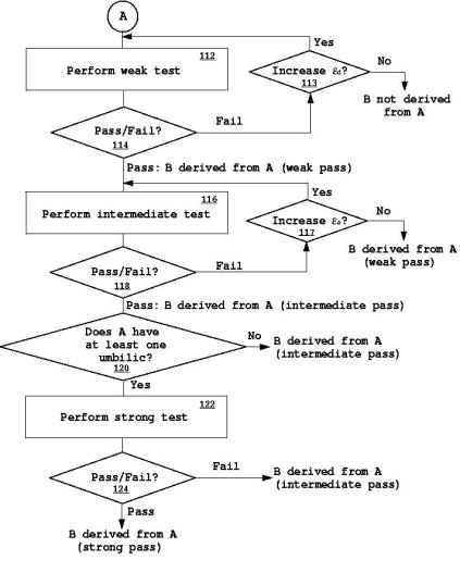
Figure 5: Algorithm 1

2.4.2. Algorithm 2

The overall procedure is the same as algorithm 1 except that no iteration is involved as shown in Figure 6. In this algorithm, a decision is made based on statistical information constructed in each step. From the weak test, statistics of the distance function are computed and evaluated by the user or a computer program. If the statistics pass a set of threshold tests, then B^’ (and B) is concluded to be derived from A under the weak test and the intermediate test begins. Otherwise, B^’ (and B) is concluded not to be derived from A.

    The intermediate test constructs statistics of intrinsic properties, i.e. angle differences of the principal directions. They are computed and evaluated by the user or a computer program. A determination is made as to whether the statistics pass a set of threshold tests. If the tests are negative, it is concluded that B^’ (and B) is derived from A under the weak test. If the tests are positive, it is concluded that B^’ (and B) is derived from A with respect to the intermediate test.

    Similarly, depending on the existence of umbilical points, the strong test may be performed. Statistics of position differences of the locations between corresponding umbilics are computed and evaluated by the user or a computer program. A determination is made as to whether the statistics pass a set of threshold tests. If the tests are negative, B^’ (and B) is concluded to be derived from A with respect to the intermediate test. If the tests are positive, it is decided that B^’ (and B) is derived from A under the strong test.

 

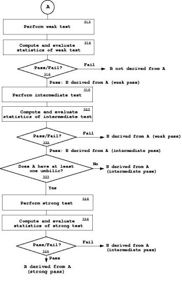
Figure 6: Algorithm 2

3. Examples

In this section, the proposed algorithms are demonstrated with various examples. Two subsections are presented: one subsection deals with examples of the proposed matching methods and the other contains an example of application to copyright protection.

3.1. Matching

3.1.1. Moment Method

Solids bounded by cubic integral B-spline surfaces, A and B are used for simplicity. Solid A is enclosed in a rectangular box of 25.0mm x 23.48mm x 11.0mm. Here, the height of solid A is 25.0mm.

 

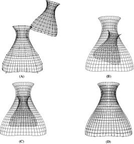
Figure 7: Matching via integral properties

 

Figure 7 shows a sequence of operations for matching of two surfaces using the principal moments of inertia of input solids. In Figure 7-(A), two boundary surfaces of the input solids are shown with the control points with them. In this example, for better visualization, only part of the boundary surfaces of each solid is displayed. The smaller solid is translated, rotated, uniformly scaled and reparameterized. Matching the centroids of mass of two solids is done by translating the small solid by the difference between the centroids, which is demonstrated in Figure 7-(B). After matching the directions of principal moment of inertia, two solids align their directions that are shown in Figure 7-(c). Figure 7-(d) shows that two solid match after the scaling value obtained by the ratio between the masses of the solids is applied to the small solid.

3.1.2. KH Method

A partial matching example using the KH method is presented in Figure 8. It shows half of a car hood which is represented by a bicubic B-spline surface patch. The hood has 64 (8 × 8) control points (enclosed in a rectangular box of 13mm × 12mm × 6mm). The smaller surface in Figure 8-(B) is a B-spline surface patch with 16 × 16 control points. The relative error after matching, i.e. the maximum distance divided by the square root of the surface area, is 0.00484.

 

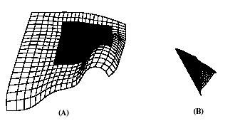
Figure 8 : A partial matching example

3.1.2. Umbilical Point Method

Suppose we have a set of data points r_A and a surface r_B as shown in Figures 9 and 10. The surface r_B shown in Figure 9 is a bicubic B-spline surface patch with 64 (8 × 8) control points enclosed in a box of 25mm×23.48mm×11mm. It has three star type umbilical points as shown in Figure 9.

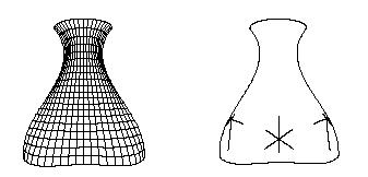
Figure 9 : Surface r_B and umbilical points

The point set r_A shown in Figure 10 is approximated with a bicubic B-spline surface patch of 256 (16×16) control points. It has one umbilical point of star type as shown in Figure 10.

 

 

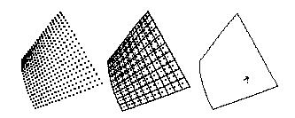
Figure 10 : Approximated surface r_A and an umbilical point

Angle distributions at the umbilical points are computed and it is found that the star type umbilical point on r_A matches the center umbilical point on r_B. Then, surface r_A is translated and rotated by using the positions of the corresponding umbilical points and the normal vectors at the umbilcal points to match surface r_B as shown in Figure 11.

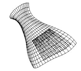
Figure 11 : Matching surfaces r_A and r_B

3.2. Copyright Protection

In this section, the two proposed similarity decision algorithms are demonstrated with the bottle example used for the moment method in Section 3.1.1. After aligning two solids A and B shown in Figure 7, we are ready to assess the similarity between them. Here, part of the bounding surfaces is used for similarity checking. The surfaces are represented as bicubic B-splines and one surface has 64 (8 × 8) and the other 144 (12×12) control points with different parametrization. Both surfaces are enclosed in a rectangular box of 25mm × 23.48mm × 11mm. The 413 node points are used from the wireframe given in Figure 4. All umbilical points for the two surfaces are located as shown in Figure 12.

 

	Umbilic 1	Umbilic 2	Umbilic 3
Distance (mm)	0.08099	0.02954	0.08115

 

Table 1: Distances between two corresponding umbilics

 

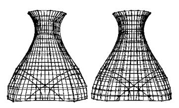
Figure 12: Comparison of lines of curvatures and umbilical points

 

In order to use Algorithm 1, we have to specify tolerances for e₀, e₁, e^’₁ and e₂. Depending on each tolerance, we can determine which test has passed or failed. Statistical information given in Table 2 is obtained for Algorithm 2. Suppose we have 0.01 as a tolerance for the weak test and subdivide the uv region into 400 square sub-regions (each box size of 0.05 × 0.05). The total number of sub-regions which contain footpoints P_i satisfying e_i > 0.01 is 31. Therefore, we can conclude that two surfaces are similar by 92.25% under the weak test with tolerance 0.01 and sub-region of size 0.05 ×0.05. This can be visualized as in Figure 13-(A). Here, the boxes indicate the regions that have at least one point with deviation larger than the tolerance 0.01. The results of the intermediate test using the maximum principal curvature are visualized in Figure 13-(B). Under the intermediate test for the maximum principal curvature with a tolerance 0.03, the similarity value between two surfaces is 91.25%. The strong test can also be performed based on the umbilical points for both surfaces as shown in Figure 12. Three star type umbilical points are identified for each surface, and the Euclidean distances between the corresponding umbilical points are calculated in Table 1. The types of the corresponding umbilical points match, and the position differences between the corresponding umbilics are small compared to the size of the objects. Therefore, we may conclude that the strong test has passed.

 

 

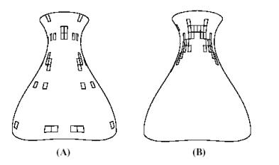
Figure 13: (A) Weak test and (B) intermediate test (maximum principal curvature)

based on Algorithm 2

 

 

Values	Distance (mm)	Max. Principal Curvature(mm-1)	Min. Principal Curvature(mm-1)
Maximum	0.03163	0.07875	0.10577
Mean	0.00852	0.01573	0.01411
Deviation	0.00004	0.00023	0.00047
Standard Deviation	0.00650	0.01533	0.02165

 

Table 2: Comparison of various quantities

 

4. Conclusions

We have addressed a problem of matching NURBS surface patches and solids bounded by NURBS surface patches, and introduced algorithms for a similarity decision. As auxiliary steps, methods of detection of umbilical points and construction of an intrinsic wireframe have been also proposed. Quantitative assessment of matching is another issue discussed in this paper. Three hierarchical tests are proposed, and two decision algorithms are developed which provide systematic and statistical measures for a user to determine the similarity between two geometric objects. The proposed matching and similarity checking techniques can be used for copyright protection of NURBS surfaces. A user can compare a suspicious surface with a surface registered with an independent repository to check if the suspect surface is a copy of the copyrighted one. The partial matching technique may provide a method to determine whether or not part of the copyrighted surface has been stolen. Similarity decision depends on user-defined tolerances. Therefore, these tolerances need to be defined by an independent party.

 

Extension of this work to deal with the problem of matching and similarity evaluation for geometric objects expressed in different representation form such as polyhedra and range data is a subject recommended for future study.

 

Acknowledgment

This work was funded by the National Science Foundation (NSF), grant number DMI-0010127.

 

References

 

[1]     O. Benedens. Geometry-based watermarking of 3-D models. IEEE Computer Graphics and Applications, 19(1):46-55, 1999.

[2]     M. V. Berry and J. H. Hannay. Umbilic points on Gaussian random surfaces. Journal of Physics A., 10(11):1809-1821, 1977.

[3]     R. T. Farouki. Graphical methods for surface differential geometry. In R. R. Martin, editor, The Mathematics of Surfaces II, pp. 363-385. Clarendon Press, 1987.

[4]     C. Fornaro and A. Sanna. Public key watermarking for authentication of CSG models. Computer Aided Design, 32(12):727-735, 2000.

[5]     R. A. Jinkerson, S. L. Abrams, L. Bardis, C. Chryssostomidis, N. M. Patrikalakis, and F.-E. Wolter. Inspection and Feature Extraction of Marine Propellers. Journal of Ship Production, 9(2):88-106, May 1993.

[6]     S. Kanai, H. Date, and T. Kishinami. Digital watermarking for 3D polygons using multiresolution wavelet decomposition. In Proceedings of the Sixth IFIP WG 5.2/GI International Workshop on Geometric Modelling: Fundamentals and Applications, Tokyo, December, 1998, pp. 296-307, 1998.

[7]     K. H. Ko, T. Maekawa, and N. M. Patrikalakis. An algorithm for optimal freeform object matching. Computer Aided Design, 35(10):913-923, September 2003.

[8]     K. H. Ko, T. Maekawa, and N. M. Patrikalakis. Algorithms for optimal partial matching of free-form objects with scaling effects. Submitted for publication, December 2002.

[9]     K. H. Ko, T. Maekawa, N. M. Patrikalakis, H. Masuda, and F.-E.Wolter. Shape intrinsic fingerprints for free-form object matching. In G. Elber and V. Shapiro, editors, 8^th ACM Symposium on Solid Modeling and Applications, pp. 196-207, Seattle, WA, June 2003.

[10]  T. Maekawa. Computation of shortest paths on free-form parametric surfaces. Journal of Mechanical Design, Transactions of the ASME, 118(4):499-508, December 1996.

[11]  T. Maekawa, N. M. Patrikalakis, F.-E. Wolter, and H. Masuda. Shape-intrinsic watermarks for 3-D solids. MIT Technology Disclosure Case 9505S, September 2001. Patent Attorney Docket No. 0050.2042-000. Application pending, January 7, 2002.

[12]  T. Maekawa, F.-E. Wolter, and N. M. Patrikalakis. Umbilics and lines of curvature for shape interrogation. Computer Aided Geometric Design, 13(2):133-161, March 1996.

[13]   R. Ohbuchi, H. Masuda, and M. Aono. Watermarking three-dimensional polygonal models through geometric and topological modifications. IEEE Journal on Selected Areas in Communications, 16(14):551-560, May 1998.

[14]   R. Ohbuchi, H. Masuda, and M. Aono. A shape-preserving data embedding algorithm for NURBS curves and surfaces. In Proceedings of Computer Graphics International, CGI '99, June 1999, pp. 180-187. IEEE Computer Society, 1999.

[15]   N. M. Patrikalakis and T. Maekawa. Shape Interrogation for Computer Aided Design and Manufacturing. Springer-Verlag, Heidelberg, February 2002.

[16]   J. Pegna and F.-E. Wolter. Surface curve design by orthogonal projection of space curves onto free-form surfaces. Journal of Mechanical Design, ASME Transactions, 118(1):45-52, March 1996.

[17]   E. Praun, H. Hoppe, and A. Finkelstein. Robust mesh watermarking. In Proceedings of SIGGRAPH '99, Los Angeles, August 8-13, 1999, pp. 49-56. ACM, 1999.

[18]   P. T. Sander and S. W. Zucker. Singularities of principal direction fields from 3-D images. In IEEE Second International Conference on Computer Vision, Tampa Florida, pp. 666-670, 1988.

[19]   E. C. Sherbrooke and N. M. Patrikalakis. Computation of the solutions of nonlinear polynomial systems. Computer Aided Geometric Design, 10(5):379-405, October 1993.

[20]   S. S. Sinha and P. J. Besl. Principal patches: A viewpoint-invariant surface description. In IEEE International Robotics and Automation, Cincinnati, Ohio, pp. 226-231, May 1990.

[21]   B. L. Yeo and M. M. Yeung. Watermarking 3D objects for verification. IEEE Computer Graphics and Applications, 19(1):36-45, 1999.

[22]   K. Yin, Z. Pan, J. Shi, and D. Zhang. Robust mesh watermarking based on multiresolution processing. Computers & Graphics, 25:409-420, 2001.

[23]   J. Zhou, E. C. Sherbrooke, and N. M. Patrikalakis. Computation of stationary points of distance functions. Engineering with Computers, 9(4):231-246, Winter 1993.