• Submit all plots and paper work with clear explanations of your work.
• E-mail your source code to trjackso@mit.edu in one file.

In this problem set, we will work with C and the graphics library OpenGL to visualize our AUV profile. The source code for a skeleton program ``graph2D'' which opens a graphics window can be copied from the 13.016 Course Locker. With comments placed in the code and the introductory lecture on OpenGL, the source code should be self-explanatory.

1. Using your favorite web browser, please go to the 13.016 home page. We will be trying to keep this site up to date with the latest information for this course (announcements, handouts, homeworks, hints, etc.). Even if you have already done so on paper, please register electronically for the course so we can create an electronic database.
2. Attach the 13.016 Course Locker. On an Athena SGI, type ``add 13.016''. With the course locker attached, you will have access to the source code and library files needed to compile graph2D.
3. Copy the source code for graph2D, examine the program, compile it, and observe what it does. The source code is kept in directory /mit/13.016/ProblemSets/PS2. Notice the source code is in several files and a Makefile is provided to simplify compilation of the code.
   Graph2D opens a viewport in which we will draw our AUV. The extents of the viewport are 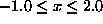, 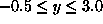which is set in the routine reshapeWindow(int w, int h). Currently, the viewport is empty.

4. Add code to the routine display() to draw x and y axes in the viewport. How you draw the axes is left up to you but please provide tick marks at regular intervals and arrow heads on the axes.
   

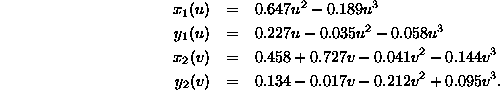
   Recall from Problem Set 1 that the upper longitudinal profile curve of the AUV is represented by two cubic planar parametric curves 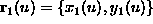and 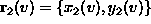, where and

   

5. Modify the display() routine to plot the profile of the AUV in the viewport. Experiment with different OpenGL primitives for representing the profile.
6. Create a ``porcupine'' plot of the curvature of the profile. This consists of evaluating the curvature at regular intervals along the profile. At each evaluation point, place a line segment at the point normal to the curve with a lengh proportional to the evaluated curvature. The constant of proportionality for this plot is a user input as well as the number of evaluation points N for each curve. For your plot, choose N=51.
7. Is the profile tangent and curvature continuous at the joint between the two curves? Determine the magnitude of the discontinuity of curvature of the two curves at their interface (connecting) point (u=1, v=0).

To make hard copies of your graphics output, use the program xv. Attach the graphics locker (type add graphics) and then type xv in an open shell. Program xv will open a separate window. Press the right mouse button in that window to get a menu of options. With your program running, press the grab button (lower right corner) and then capture your window as an image. With the image captured, you can either print directly or save the image as a postscript file. Use xv to make hard copies of the output of your program in different development stages (axes only; axes and profile; axes, profile, and porcupine; or any other experimenting you feel inclined to do).