Use the program evaluate in the directory
/mit/13.016/ProblemSets/PS5/Subdivide to split the Bézier curve into three smaller Bézier curves. The three Bézier curves are generated by splitting the curve at parametric value followed by splitting the second of the resulting curves at ( its own) parametric value .

Turn in a list of the control points of the initial curve, the two intermediate curves, and the final three curves. Also, create a plot of the initial, intermediate, and final control polygons of the Bézier curves, and of the initial Bézier curve evaluated at 100 evenly distributed points using the same algorithm. Use OpenGL in creating your plots. Turn in your code and results via e-mail to trjackso@mit.edu.

• Set the viewpoint at (5.0,5.0,5.0), and then rotate about the view direction by . Use orthographic projection first, and then change to perspective projection.
• For the following three transformations, different sequences result in different objects. Try the sequences a-b-c, b-c-a, and c-a-b, and turn in your plots:
  1. Scale the x-axis of the modeling space by 2 .
  2. Rotate the modeling space first around the x-axis by , and then around the y-axis by .
  3. Translate the modeling space by .

A skeleton program called `xform_cube' to get you started is provided in the course locker, /mit13.016/ProblemSets/PS5.

Hand in your plots illustrating the different sequences and submit your source code via email to trjackso@mit.edu.

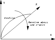
Let us define the profile of the AUV in terms of Bézier curves and which specify the radius of the curve at the corresponding longitudinal position. The control points for the profile curves are

The surface of an AUV can be described by revolving the profile around the x -axis. Mathematically, this can be expressed as

where , , and is the angle measured from the xy plane.

1. Illustrate each of the two surfaces by a perspective projection of a grid of isoparameter lines. The code from Problem 1 for evaluating points on Bézier curves should be used at this point.
2. Provide an analytical expression for the unit normal vector of each of the surfaces ( and ).
3. Render the surface of the AUV. To get the correct shading, you will need to evaluate the normals from above.

A skeleton program called `vis_auv' to get you started is provided in the course locker, /mit13.016/ProblemSets/PS5.

Hand in plots illustrating your wirefame and surface rendering of the AUV and paper work showing your calculation of the unit normals of the surfaces. Submit your source code via email to trjackso@mit.edu.